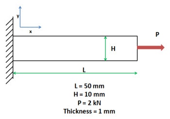
Problem Specification

A steel bar is mounted in a rigid wall and axially loaded at the end by a force P = 2 kN as shown in the figure below. The bar dimensions are indicated in the figure. The bar is so thin that there is no significant stress variation through the thickness. Neglect gravity.

In this exercise, you are presented with the numerical solution to the above problem obtained from finite-element analysis (FEA) using ANSYS software.Compare FEA results for the stress distribution presented to you with the corresponding analytical solution. Justify agreements and discrepancies between the two approaches (FEA vs. Analytical).

Note that you will be using the ANSYS solution presented to you to explore the physics of the problem. You will be downloading the ANSYS solution prepared for you. The objective is to help you learn important fundamentals of mechanics through the interactive, visual interface provided by ANSYS. You will not be obtaining the FEA solution using ANSYS; there are other tutorials to help you learn this. 

Pre-Analysis and Start-Up

Since we don't expect significant variation of stresses in the z direction, it is reasonable to assume plane stress: 

The deformed structure will be in equilibrium. Thus, the 2D stress components should satisfy the 2D equilibrium equations: 

We need to solve these equations in our rectangular domain and impose the appropriate boundary conditions: imposed displacement constraints at the left end and applied force at the right end. In effect, we have to solve a boundary value problem (BVP). Recall that the elements of a BVP are:

• Governing differential equations 
• Domain
• Boundary conditions

You probably have solved simple BVPs before in your math classes. We will first review the analytical approach to solving this BVP. We'll then look at the FEA approach. 

Analytical Solution

Since we are ignoring the effects of gravity; there are no body forces per unit volume.

Since the length is much larger than the width, we ignore end effects and neglect variations in the y direction. Plugging and chugging into the equilibrium equations yields

Then the equilibrium equation in the x-direction becomes:

Therefore,

Apply Boundary Conditions: If we make a vertical cut in the geometry, then the stress must be P/A. Therefore, 

 This is of course a well-known result. For this problem, we have 

Numerical Solution using FEA

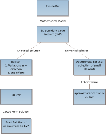
In the numerical solution using FEA, we solve the 2D BVP directly by dividing the structure into small elements and approximating the solution for these small elements. Unlike the analytical approach, we do not assume that there is no variation in the y direction. Also, end effects are not neglected. The FEA solution is an approximate solution to the 2D BVP. The approximation gets better as the elements become smaller. In contrast, the analytical solution presented above is the exact solution to the 1D BVP obtained by making approximations to the 2D BVP. In other words, in the analytic solution, we have swapped the actual 2D BVP problem for a 1D BVP problem that we can solve in closed form. Both approaches have value in engineering and complement each other. We have checked that the FEA solution presented to you is reasonably accurate. 

The following figure summarizes the contrasts between the analytical and numerical approaches.

 

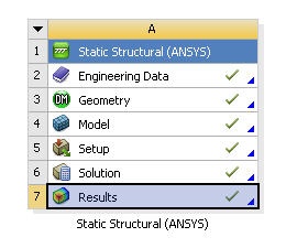
Load FEA Solution obtained using ANSYS

As mentioned before, we are providing the FEA solution obtained using ANSYS so that you can focus on comparing the analytical and numerical solutions (which is the goal of this exercise). Without further ado, let's download the ANSYS solution and load it into ANSYS.

1. Download "Tensile Bar Demo.zip" by clicking here
The zip should contain a Tensile Bar Demo folder with the following contents:
- Tensile Bar Demo_files folder
- Tensile Bar Demo.wbpj
Please make sure both these are in the folder, otherwise the solution will not load into ANSYS properly. (Note: The solution provided was created using ANSYS workbench 13.0 release, there may be compatibility issues when attempting to open with other versions). Be sure to extract before use.

2. Double click "Tensile Bar Demo.wbpj" - This should automatically open ANSYS Workbench (you have to twiddle your thumbs a bit before it opens up). You will then be presented with the ANSYS solution in the project page.

A tick mark against each step indicates that that step has been completed.

3. To look at the results, double click on Results - This should bring up a new window (again you have to twiddle your thumbs a bit before it opens up).

4. On the left-hand side there should be an Outline toolbar. Look for Solution (A6).

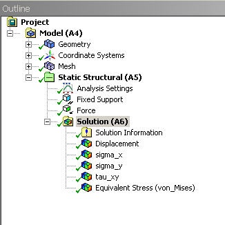
Results

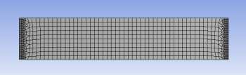
Before we explore the ANSYS results, let's take a peek at the mesh.

Mesh

Click on Mesh (above Solution) in the tree outline. This shows the mesh used to generate the ANSYS solution. The domain is a rectangle. This domain is discretized into a number of small "elements". For each element, ANSYS approximates how the structure responds to the forces acting on the element. A finer mesh is used in areas of greater stress concentration. We have checked that the solution presented  to you is reasonably independent of the mesh.

 

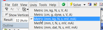
Units

Set the units for the results display by selecting Units > Metric (mm, kg, N, s, mV, mA). The displacements will be reported in mm and the stresses in N/mm2 which is equivalent to MPa.

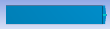
Displacement

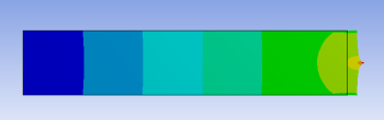
To view the deformed structure, click on Solution > Displacement in the tree outline. The black rectangle shows the undeformed structure. The deformed structure is colored by the magnitude of the displacement. Red areas have deformed more and blue areas less. You can see that the left end has not moved as specified in the problem statement. This means this boundary condition has been applied correctly. The displacement increases from left to right as we intuitively expect. There is also not much variation in the y-direction. So we can conclude that the model has been constrained properly.

Note the extremely high deformation near the point load. This extremum is unrealistic and should be ignored (there are no point loads in reality).

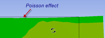
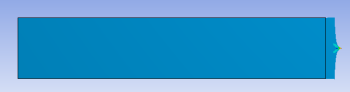
To view the Poisson effect (shrinking in the y direction), zoom into the top-rightright corner by drawing a rectangle around the region with the right mouse button.

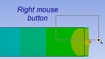
You can do this multiple times to zoom in more. You do indeed see the shrinking in the y-direction as expected but it is small for this model.

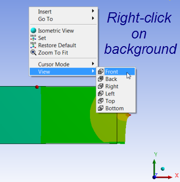
You can restore the front view of the entire model by right-clicking in the background and choosing View > Front.

If you zoom into the top-left corner, you will see that the model cannot shrink in the y-direction at the left boundary where it is fixed. In other words, it "wants to" shrink in the y-direction at the top-left corner but cannot due to the displacement constraint we impose. So can expect a stress concentration near this corner.

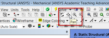
Note that you can zoom in and out using the middle mouse wheel. You can translate the model by clicking on the Pan button and dragging the model with the left mouse button. There are also a bunch of zoom options next to the Pan button.

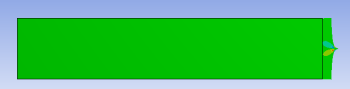
sigma_x

Next, let's take a look at the stress components starting with sigma_x. Click on Solution > sigma_x in the tree outline. The stress is uniform away from the ends. To check what the value is in the uniform region, click on Probe in the toolbar (see snapshot below) at the top and move the cursor on the structure; Probe values in the middle as well as at the ends. You may need to translate the model to the right to see the probe values near the left end.

 

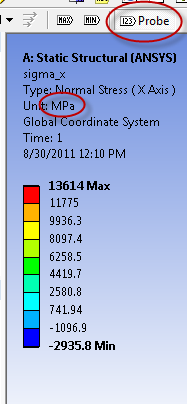
The value of sigma_x away from the ends is nearly 200 MPa (the unit is indicated above the plot). This matches with the P/A value expected from the Pre-Analysis step.

 

In the sigma_x plot, we see that there is deviation from the analytical value in two regions:

• Around the point load (again the extremely high values very close to the point load are unrealistic).
• At the fixed end.

The analytical solution is inaccurate in these regions since the 1D assumption breaks down. In fact, as the mesh is refined further, the stress at the point load will approach infinity. 

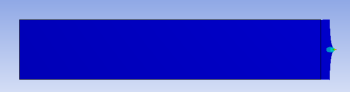
sigma_y

Next, let's take a look at sigma_y. Click on Solution > sigma_y in the tree outline. Again, probe values in the middle as well as at the ends. The value in the middle is close to zero as expected from the analytical solution. There is significant deviation from the analytical solution at both ends. Note that there are areas where sigma_y is negative i.e. compressive.

tau_xy

We expect tau_xy to be zero away from the ends. Near the ends, since sigma_x and sigma_y are non-zero, we expect 

Plot tau_xy, look at the range of values and use Probe to check actual values. Are the above statements valid?

Equivalent Stress (Von Mises):

The Equivalent or Von Mises stress is used to predict yielding of the material. We can consider the maximum and minimum equivalent stresses as the critical design points. We can see that the analytical solution under-predicts the maximum equivalent stress. Thus, one would need to use a large factor of safety if using the analytical result while designing such a structure. One would use a factor of safety with the FEA result also but it does not have to be as large.