Sunday, 24 February 2013
Saturday, 23 February 2013
Problem Specification
A curved beam with a rectangular cross section is subjected to a moment of 300 inch-pounds. The curved beam has an inner radius of 10 inches and outer radius of 12 inches. The beam is .25 inches thick.
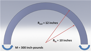
Calculate the stresses at r = 11.5 inches.
In this exercise, you are presented with the numerical solution to the above problem obtained from finite-element analysis (FEA) using ANSYS software. Compare FEA results for the stress distribution presented to you with the corresponding analytical solution. Justify agreements and discrepancies between the two approaches (FEA vs. Analytical).
Note that you will be using the ANSYS solution presented to you to explore the physics of the problem. You will be downloading the ANSYS solution prepared for you. The objective is to help you learn important fundamentals of mechanics through the interactive, visual interface provided by ANSYS. You will not be obtaining the FEA solution using ANSYS; there are other tutorials to help you learn this.
Pre-Analysis & Start-Up
Pre-Analysis
There are three difference theories for finding the solution for the bending of a curved beam. There is elasticity theory, where

There is Winkler Bach Theory, where
And there is the straight beam theory, where
ANSYS Simulation
Now, let's load the problem into ANSYS and see how a computer simulation will compare. First, start by downloading the files here
The zip file should contain the following contents:
The zip file should contain the following contents:
- Curved Beam Solution_files folder
- Curved Beam Solution.wbpj
Please make sure to extract both of these files from the zip folder, the program will not work otherwise. (Note: The solution was created using ANSYS workbench 12.1 release, there may be compatibility issues when attempting to open with other versions).
2. Double click "Curved Beam Solution.wbpj" - This should automatically open ANSYS workbench (you have to twiddle your thumbs a bit before it opens up). You will be presented with the ANSYS solution.
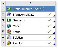
A tick mark against each step indicates that that step has been completed.
3. To look at the results, double click on "Results" - This should bring up a new window (again you have to twiddle your thumbs a bit before it opens up).
4. On the left-hand side there should be an "Outline" toolbar. Look for "Solution (A6)".
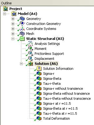
Tuesday, 19 February 2013
Problem Specification
A steel bar is mounted in a rigid wall and axially loaded at the end by a force P = 2 kN as shown in the figure below. The bar dimensions are indicated in the figure. The bar is so thin that there is no significant stress variation through the thickness. Neglect gravity.
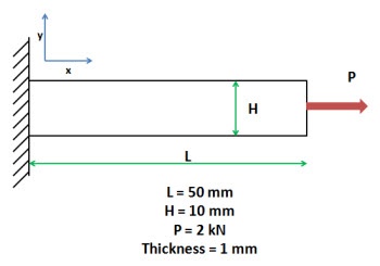
In this exercise, you are presented with the numerical solution to the above problem obtained from finite-element analysis (FEA) using ANSYS software.Compare FEA results for the stress distribution presented to you with the corresponding analytical solution. Justify agreements and discrepancies between the two approaches (FEA vs. Analytical).
Note that you will be using the ANSYS solution presented to you to explore the physics of the problem. You will be downloading the ANSYS solution prepared for you. The objective is to help you learn important fundamentals of mechanics through the interactive, visual interface provided by ANSYS. You will not be obtaining the FEA solution using ANSYS; there are other tutorials to help you learn this.
Note that you will be using the ANSYS solution presented to you to explore the physics of the problem. You will be downloading the ANSYS solution prepared for you. The objective is to help you learn important fundamentals of mechanics through the interactive, visual interface provided by ANSYS. You will not be obtaining the FEA solution using ANSYS; there are other tutorials to help you learn this.
Pre-Analysis and Start-Up
Since we don't expect significant variation of stresses in the z direction, it is reasonable to assume plane stress:

The deformed structure will be in equilibrium. Thus, the 2D stress components should satisfy the 2D equilibrium equations:

We need to solve these equations in our rectangular domain and impose the appropriate boundary conditions: imposed displacement constraints at the left end and applied force at the right end. In effect, we have to solve a boundary value problem (BVP). Recall that the elements of a BVP are:
- Governing differential equations
- Domain
- Boundary conditions
You probably have solved simple BVPs before in your math classes. We will first review the analytical approach to solving this BVP. We'll then look at the FEA approach.
Analytical Solution
Since we are ignoring the effects of gravity; there are no body forces per unit volume.

Since the length is much larger than the width, we ignore end effects and neglect variations in the y direction. Plugging and chugging into the equilibrium equations yields

Then the equilibrium equation in the x-direction becomes:

Therefore,

Apply Boundary Conditions: If we make a vertical cut in the geometry, then the stress must be P/A. Therefore,

This is of course a well-known result. For this problem, we have

Numerical Solution using FEA
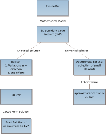
In the numerical solution using FEA, we solve the 2D BVP directly by dividing the structure into small elements and approximating the solution for these small elements. Unlike the analytical approach, we do not assume that there is no variation in the y direction. Also, end effects are not neglected. The FEA solution is an approximate solution to the 2D BVP. The approximation gets better as the elements become smaller. In contrast, the analytical solution presented above is the exact solution to the 1D BVP obtained by making approximations to the 2D BVP. In other words, in the analytic solution, we have swapped the actual 2D BVP problem for a 1D BVP problem that we can solve in closed form. Both approaches have value in engineering and complement each other. We have checked that the FEA solution presented to you is reasonably accurate.
The following figure summarizes the contrasts between the analytical and numerical approaches.
Load FEA Solution obtained using ANSYS
As mentioned before, we are providing the FEA solution obtained using ANSYS so that you can focus on comparing the analytical and numerical solutions (which is the goal of this exercise). Without further ado, let's download the ANSYS solution and load it into ANSYS.
1. Download "Tensile Bar Demo.zip" by clicking here
The zip should contain a Tensile Bar Demo folder with the following contents:
- Tensile Bar Demo_files folder
- Tensile Bar Demo.wbpj
Please make sure both these are in the folder, otherwise the solution will not load into ANSYS properly. (Note: The solution provided was created using ANSYS workbench 13.0 release, there may be compatibility issues when attempting to open with other versions). Be sure to extract before use.
2. Double click "Tensile Bar Demo.wbpj" - This should automatically open ANSYS Workbench (you have to twiddle your thumbs a bit before it opens up). You will then be presented with the ANSYS solution in the project page.
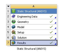
A tick mark against each step indicates that that step has been completed.

A tick mark against each step indicates that that step has been completed.
3. To look at the results, double click on Results - This should bring up a new window (again you have to twiddle your thumbs a bit before it opens up).
4. On the left-hand side there should be an Outline toolbar. Look for Solution (A6).
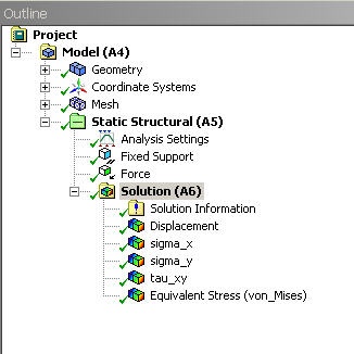
Results
Before we explore the ANSYS results, let's take a peek at the mesh.
Mesh
Click on Mesh (above Solution) in the tree outline. This shows the mesh used to generate the ANSYS solution. The domain is a rectangle. This domain is discretized into a number of small "elements". For each element, ANSYS approximates how the structure responds to the forces acting on the element. A finer mesh is used in areas of greater stress concentration. We have checked that the solution presented to you is reasonably independent of the mesh.

Units
Set the units for the results display by selecting Units > Metric (mm, kg, N, s, mV, mA). The displacements will be reported in mm and the stresses in N/mm2 which is equivalent to MPa.

Displacement
To view the deformed structure, click on Solution > Displacement in the tree outline. The black rectangle shows the undeformed structure. The deformed structure is colored by the magnitude of the displacement. Red areas have deformed more and blue areas less. You can see that the left end has not moved as specified in the problem statement. This means this boundary condition has been applied correctly. The displacement increases from left to right as we intuitively expect. There is also not much variation in the y-direction. So we can conclude that the model has been constrained properly.
Note the extremely high deformation near the point load. This extremum is unrealistic and should be ignored (there are no point loads in reality).

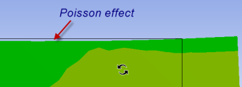
To view the Poisson effect (shrinking in the y direction), zoom into the top-rightright corner by drawing a rectangle around the region with the right mouse button.
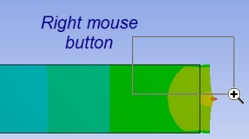
You can do this multiple times to zoom in more. You do indeed see the shrinking in the y-direction as expected but it is small for this model.
You can restore the front view of the entire model by right-clicking in the background and choosing View > Front.
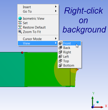
If you zoom into the top-left corner, you will see that the model cannot shrink in the y-direction at the left boundary where it is fixed. In other words, it "wants to" shrink in the y-direction at the top-left corner but cannot due to the displacement constraint we impose. So can expect a stress concentration near this corner.
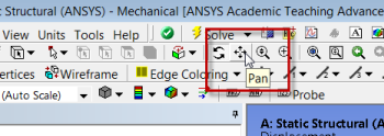
Note that you can zoom in and out using the middle mouse wheel. You can translate the model by clicking on the Pan button and dragging the model with the left mouse button. There are also a bunch of zoom options next to the Pan button.
sigma_x
Next, let's take a look at the stress components starting with sigma_x. Click on Solution > sigma_x in the tree outline. The stress is uniform away from the ends. To check what the value is in the uniform region, click on Probe in the toolbar (see snapshot below) at the top and move the cursor on the structure; Probe values in the middle as well as at the ends. You may need to translate the model to the right to see the probe values near the left end.
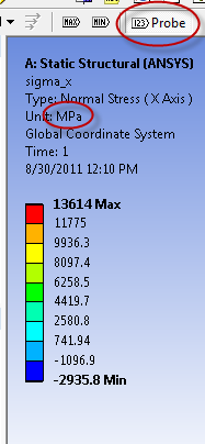
The value of sigma_x away from the ends is nearly 200 MPa (the unit is indicated above the plot). This matches with the P/A value expected from the Pre-Analysis step.

In the sigma_x plot, we see that there is deviation from the analytical value in two regions:
- Around the point load (again the extremely high values very close to the point load are unrealistic).
- At the fixed end.
The analytical solution is inaccurate in these regions since the 1D assumption breaks down. In fact, as the mesh is refined further, the stress at the point load will approach infinity.
sigma_y
Next, let's take a look at sigma_y. Click on Solution > sigma_y in the tree outline. Again, probe values in the middle as well as at the ends. The value in the middle is close to zero as expected from the analytical solution. There is significant deviation from the analytical solution at both ends. Note that there are areas where sigma_y is negative i.e. compressive.

tau_xy
We expect tau_xy to be zero away from the ends. Near the ends, since sigma_x and sigma_y are non-zero, we expect

Plot tau_xy, look at the range of values and use Probe to check actual values. Are the above statements valid?

Equivalent Stress (Von Mises):
The Equivalent or Von Mises stress is used to predict yielding of the material. We can consider the maximum and minimum equivalent stresses as the critical design points. We can see that the analytical solution under-predicts the maximum equivalent stress. Thus, one would need to use a large factor of safety if using the analytical result while designing such a structure. One would use a factor of safety with the FEA result also but it does not have to be as large.

Monday, 18 February 2013
Referring to Section 17.1.3 of the ABAQUS User's manual you will require the heat transfer properties as well as the electrical properties. These are listed below :
This forms the complete set of properties. If Piezoelectric elements are not used then *PIEZOELECTRIC and *DIELECTRIC properties will not be required.
If only the steady state heat transfer response is of interest then *SPECIFIC HEAT properties are not required. Similarly if there are no phase changes involved then *LATENT HEAT is not required.
*JOULE HEAT FRACTION is used to specify the fraction of electrical energy that will be released as heat.
Example problem 5.2.1 - thermal-electrical modelling of an automotive fuse illustrates the thermal-electrical analysis.
ABAQUS allows for redundant material properties to be specified. It will simply ignore the material properties not required for the current analysis.
Typical example of material properties :
- Heat Transfer properties
- *CONDUCTIVITY
- *LATENT HEAT
- *SPECIFIC HEAT
- *HEAT GENERATION
- Electrical properties
- *DIELECTRIC
- *ELECTRICAL CONDUCTIVITY
- *JOULE HEAT FRACTION
- *PIEZOELECTRIC
This forms the complete set of properties. If Piezoelectric elements are not used then *PIEZOELECTRIC and *DIELECTRIC properties will not be required.
If only the steady state heat transfer response is of interest then *SPECIFIC HEAT properties are not required. Similarly if there are no phase changes involved then *LATENT HEAT is not required.
*JOULE HEAT FRACTION is used to specify the fraction of electrical energy that will be released as heat.
Example problem 5.2.1 - thermal-electrical modelling of an automotive fuse illustrates the thermal-electrical analysis.
ABAQUS allows for redundant material properties to be specified. It will simply ignore the material properties not required for the current analysis.
Typical example of material properties :
*MATERIAL, NAME=ZINC
*CONDUCTIVITY
 0.1121,  20.0
 0.1103, 100.0
*ELECTRICAL CONDUCTIVITY
 16.75E3,  20.0
 12.92E3, 100.0
*JOULE HEAT FRACTION
  1.0
*DENSITY
  7.14E-6
*SPECIFIC HEAT
  389.0
Referring to Section 17.1.3 of the ABAQUS User's manual you will require the heat transfer properties as well as the mechanical properties. These are listed below :
- Mechanical properties
- *ELASTIC
- Additional properties which may be required : example plastic
- Heat Transfer properties
- *CONDUCTIVITY
- *LATENT HEAT
- *SPECIFIC HEAT
- *HEAT GENERATION
Read the relevant section in Chapter 6 : Analysis Procedures (User's manual Vol. I). This gives an overview about the analysis and has more information about the material properties.
Read also the following sections in Chapter 17 : Materials Introduction of the ABAQUS User's manual.
Section 17.1.3 lists the material model combination tables. Several models are available to define the mechanical behaviour (elastic, plastic).
Some material options require the presence of other material options. Some exclude the use of the other material options. For example *DEFORMATION PLASTICITY completely defines the material's mechanical behaviour and should not be used with *ELASTIC.
Once you have all the relevant keywords to define the material properties consult the keyword Manual for each of the keywords. This will explain what data is required for each of the keyword.
Read also the following sections in Chapter 17 : Materials Introduction of the ABAQUS User's manual.
- Section 17.1.1 - Material Library : Overview
- Section 17.1.2 - Material Data Definition
- Section 17.1.3 - Combining Material Properties
Section 17.1.3 lists the material model combination tables. Several models are available to define the mechanical behaviour (elastic, plastic).
Some material options require the presence of other material options. Some exclude the use of the other material options. For example *DEFORMATION PLASTICITY completely defines the material's mechanical behaviour and should not be used with *ELASTIC.
Once you have all the relevant keywords to define the material properties consult the keyword Manual for each of the keywords. This will explain what data is required for each of the keyword.
Sunday, 17 February 2013
Use the concrete model available with rebar to model the reinforcements.
Section 1.1.5 of the ABAQUS Example's manual gives an example of the collapse analysis of a concrete slab subjected to a central point load.
The data file for that example is collapse example.
The complete set of ABAQUS input files can be obtained by using the following command :
This is used to define the shape of the failure surface (see section 11.5.1 of the ABAQUS USER's manual Vol. II).
The first parameter is the ratio of the ultimate biaxial compression stress, to theuniaxial compressive stress. Default is 1.16.
The second parameter is the absolute value of the ratio of uniaxial tensile stressat failure to the uniaxial compressive stress at failure. Default is 0.09.
First parameter is the fraction of remaining stress to stress at cracking. The second parameter is the absolute value of the direct strain minus the direct strain at cracking.
This defines the retained tensile stress normal to the crack as a function of the deformation in the direction of the normal to the crack.
*REBAR is used to model the reinforcement.
Here SLAB is the element name or name of the element set that contains these rebars. The geometry is ISOPARAMETRIC. Other choice is SKEW. ELEMENT can be BEAM, SHELL, AXISHELL or CONTINUUM type. The following are the other parameters specified :
Section 1.1.5 of the ABAQUS Example's manual gives an example of the collapse analysis of a concrete slab subjected to a central point load.
The data file for that example is collapse example.
The complete set of ABAQUS input files can be obtained by using the following command :
abaqus fetch j=collapseconcslab*
*CONCRETE
  3000., 0.      abs. value of compressive stress, abs. value of plastic strain.
  5500., 0.0015                "                              "

*FAILURE RATIOS
  1.16, 0.0836
This is used to define the shape of the failure surface (see section 11.5.1 of the ABAQUS USER's manual Vol. II).
The first parameter is the ratio of the ultimate biaxial compression stress, to theuniaxial compressive stress. Default is 1.16.
The second parameter is the absolute value of the ratio of uniaxial tensile stressat failure to the uniaxial compressive stress at failure. Default is 0.09.
Tension Stiffening
*TENSION STIFFENING
  1., 0.
  0., 2.E-3
First parameter is the fraction of remaining stress to stress at cracking. The second parameter is the absolute value of the direct strain minus the direct strain at cracking.
This defines the retained tensile stress normal to the crack as a function of the deformation in the direction of the normal to the crack.
Shear Retention
*SHEAR RETENTIONNot used for this example.
Reinforcement modelling
*REBAR is used to model the reinforcement.
*REBAR,ELEMENT=SHELL,MATERIAL=SLABMT,GEOMETRY=ISOPARAMETRIC,NAME=YY
SLAB, 0.014875, 1., -0.435, 4
*REBAR,ELEMENT=SHELL,MATERIAL=SLABMT,GEOMETRY=ISOPARAMETRIC,NAME=XX
SLAB, 0.014875, 1., -0.435, 1
Here SLAB is the element name or name of the element set that contains these rebars. The geometry is ISOPARAMETRIC. Other choice is SKEW. ELEMENT can be BEAM, SHELL, AXISHELL or CONTINUUM type. The following are the other parameters specified :
- cross-sectional area of the rebar.
- spacing of the rebars in the plane of the shell
- position of the rebar. Distance from the reference surface. Here the mid-surface is the reference surface and the minus sign indicates that the distance is measured in the opposite direction to the direction of positive normal. The positive normal is defined by the right hand rule as the nodes are considered in an anti-clockwise sequence.
- edge number to which rebars are similar.
Alternate Method of modelling REBAR Reinforcements
Alternatively REBAR can be modelled as follows :*NODE
....
....
**-------------------END NODES FOR REBAR BEAM ELEMENTS
501, 0.0, 0.15, -0.02
541, 1.5, 0.15, -0.02
601, 0.0, 0.15, -0.07
641, 1.5, 0.15, -0.07
701, 0.0, 0.60, -0.02
741, 1.5, 0.60, -0.02
801, 0.0, 0.60, -0.07
841, 1.5, 0.60, -0.07
....
....
**---------------------GENERATE INTERMEDIATE NODES
*NGEN, NSET=BAR10TF
701, 741, 2
*NGEN, NSET=BAR10TB
801, 841, 2
...
...
**--------------------GENERATE THE BEAM ELEMENTS
*ELEMENT, TYPE=B31
701, 701, 703
801, 801, 803
*ELGEN, ELSET=BAR10TF
701, 20, 2, 1, 1, 1, 1
*ELGEN, ELSET=BAR10TB
801, 20, 2, 1, 1, 1, 1
...
...
**---------------------DEFINE THE MATERIAL PROPERTIES
*MATERIAL, NAME=BAR8
**
** 8 mm dia bar
**
*ELASTIC, TYPE=ISO
197.E6, 0.3
*PLASTIC
354.E3, 0.
364.E3, 0.0018
**
**---------------------DEFINE THE SECTION PROPERTIES
...
...
*BEAM SECTION, SECTION=CIRC, MATERIAL=BAR10, ELSET=BAR10TF
0.005
*BEAM SECTION, SECTION=CIRC, MATERIAL=BAR10, ELSET=BAR10TB
0.005
...
**--------------------DEFINE AN ELEMENT SET WHICH CONTAINS
**--------------------THE ELEMENTS THROUGH WHICH THE REBAR
**--------------------ELEMENTS PASSES.
....
*ELSET, ELSET=TOP, GENERATE
5, 80, 5
**
**--------------------
*EMBEDDED ELEMENT,HOST ELSET=TOP
BAR10TF,BAR10TB
**
Referring to Section 9.1.3 of the ABAQUS User's manual you will require theelectrical properties. These are listed below :
- Electrical properties
- *DIELECTRIC
- *ELECTRICAL CONDUCTIVITY
- *JOULE HEAT FRACTION
- *PIEZOELECTRIC
In the Mesh Module choose Mesh -> Element Type and in the dialog box which appears the default element type will listed in the bottom. Make the necessary changes as to choice of Order, Reduced integration and for some element types select Incompatible Mode if using the lower order quadrilateral or 3-D solid to model that involves bending.
Tuesday, 5 February 2013
Yes it is possible to scale the Geometry when it is read into the CAE program. Select the appropriate input using File --> Import --> Part
Change the File type to the appropriate depending on the format. Select the file and click on OK. In the form that pops up click on the Scale TAB and set the toggle key for Multiply all lengths and enter an appropriate scale factor value.
Change the File type to the appropriate depending on the format. Select the file and click on OK. In the form that pops up click on the Scale TAB and set the toggle key for Multiply all lengths and enter an appropriate scale factor value.
Yes. Use the TIE option available under MPC (Multi Point Constraint) to tie the respective nodes as illustrated in the figure below :

This would then treat these pair of nodes as identical ie. they will have the same nodal variables. This can also be useful in situations where the mesh used in an axisymmetric analysis is generated from a single surface wrapped around (rather than using the axisymmetric elements available in ABAQUS). See figure below. Then the TIE option could be used along line joining the 2 edges (and the 2 sets of nodes).

If there are several such nodes these could be grouped together into sets and the TIE option specified with a single data line. Here the corresponding nodes should appear in the correct order.
*MPC
TIE,  100, 200
TIE,  101, 201
         ......
TIE,  104, 204
This would then treat these pair of nodes as identical ie. they will have the same nodal variables. This can also be useful in situations where the mesh used in an axisymmetric analysis is generated from a single surface wrapped around (rather than using the axisymmetric elements available in ABAQUS). See figure below. Then the TIE option could be used along line joining the 2 edges (and the 2 sets of nodes).
If there are several such nodes these could be grouped together into sets and the TIE option specified with a single data line. Here the corresponding nodes should appear in the correct order.
*NSET, NSET=TOP
 100,  101,  102,  103,  104
*NSET, NSET=BOT
 200,  201,  202,  203,  204
*MPC
 TIE, TOP, BOT
Use the FORTRAN program given below to scale the X, Y and Z by factors xf, yf anf zf automatically. It will prompt for the ABAQUS input file name. The output file name will be created by appending "new" to the file name.
The program has been tested with ifort in the Linux system, f90 in the HP System and also with Force 2.0 in the Windows PC XP system.
Fortran Program to scale X, Y and Z co-ordinates.
The program has been tested with ifort in the Linux system, f90 in the HP System and also with Force 2.0 in the Windows PC XP system.
Fortran Program to scale X, Y and Z co-ordinates.
Element defnition for the spring element :*Element, type=Spring2, elset=Springs/Dashpots-1-spring
1, Bay1GroundFloor.5, Part-2-1.1
2, Bay1GroundFloor.7, Part-2-1.4
3, Bay1GroundFloor.8, Part-2-1.6
4, Bay1GroundFloor.3, Part-2-1.2
The spring stiffness is*Spring, elset=Springs/Dashpots-1-spring
2, 2
**
** spring stiffness
**
7.8E+06,
By adding the nonlinear one could then define Spring behaviour which is different for compression and tension.*Spring, elset=Springs/Dashpots-1-spring, nonlinear
2, 2
**
** Force1, Rel. Displacement-1
** Force2, Rel. Displacemnet-2
**
10.E8, -0.1
10.E6, -0.001
0, 0
7.8E+06, 1.0
1, Bay1GroundFloor.5, Part-2-1.1
2, Bay1GroundFloor.7, Part-2-1.4
3, Bay1GroundFloor.8, Part-2-1.6
4, Bay1GroundFloor.3, Part-2-1.2
2, 2
**
** spring stiffness
**
7.8E+06,
2, 2
**
** Force1, Rel. Displacement-1
** Force2, Rel. Displacemnet-2
**
10.E8, -0.1
10.E6, -0.001
0, 0
7.8E+06, 1.0
In the Mesh module click on the Element Type icon. In the dialog box which appears choose the element order you require (from the available list : Linear, Quadratic)
If using the quadratic (2D) and Hex elements (3D) choose Incompatible Modeelements if using the lower order elements.
First of all one need to specify local cylindrical co-ordinate system because of the geometry. Figure 3.6 shows the Global co-ordinate system. The axial direction (Z') is in the direction of the Global X-axis.
*ORIENTATION, SYSTEM=CYLINDRICAL, NAME=CYLIND < xa >, < ya > , < za > , < xb >, < yb > , < zb > < normal-axis > , < rotation angle >
For the above system, this will be *ORIENTATION, SYSTEM=CYLINDRICAL, NAME=CYLIND 0, 0, 0, 1, 0, 0 1, 0
The next line indicates which of the 3 (Local) axes is normal to the cylindrical surface. This is X' (Radial) axis (which is axis 1). Then the next number is the rotation about the normal axes if re-orientation is required in specifying the material directions. Any rotation applied will be counter-clockwise
Without any rotation the other 2 axes (Y' and Z') form the local directions. Y' and Z' become the material 1 and 2 directions respectively.
Referring to Figure 3.6 The Blue (circumferential line) is the material - 1 direction. The Cyan (axial) line is the material - 2 direction.

Material directions
Let us assume that the composite is made up of 3 plies which are +10, 0 -10 degrees to the cylindrical direction.
Then the composite shell will be specified as follows :

*ORIENTATION, SYSTEM=CYLINDRICAL, NAME=CYLIND < xa >, < ya > , < za > , < xb >, < yb > , < zb > < normal-axis > , < rotation angle >
For the above system, this will be *ORIENTATION, SYSTEM=CYLINDRICAL, NAME=CYLIND 0, 0, 0, 1, 0, 0 1, 0
The next line indicates which of the 3 (Local) axes is normal to the cylindrical surface. This is X' (Radial) axis (which is axis 1). Then the next number is the rotation about the normal axes if re-orientation is required in specifying the material directions. Any rotation applied will be counter-clockwise
Without any rotation the other 2 axes (Y' and Z') form the local directions. Y' and Z' become the material 1 and 2 directions respectively.
Referring to Figure 3.6 The Blue (circumferential line) is the material - 1 direction. The Cyan (axial) line is the material - 2 direction.
Material directions
Let us assume that the composite is made up of 3 plies which are +10, 0 -10 degrees to the cylindrical direction.
Then the composite shell will be specified as follows :
**
*ORIENT**
*SHELL SECTION, ELSET=CYLIND, COMPOSITE, ORIENTATION=ORI
0.05, , WOVEN,  10
0.05, , PLYTRON, 0
0.05, , PLYTRON, 0
*ORIENTATION, SYSTEM=CYLINDRICAL, NAME=ORILet us consider another situation where the zero ply direction is aligned to the axial direction. The other 2 ply directions 30 degrees either side of this direction. In this situation it is preferrable to have the material-1 direction to be the axial direction. This is done by applying an additional rotation of 90 about the normal.
0,0,0,0,0,1
1,0
**
**
*SHELL SECTION, ELSET=CYLIND, COMPOSITE, ORIENTATION=ORI
0.05, , WOVEN, -45
0.05, , PLYTRON, 90
0.05, , PLYTRON, 0
**
*ORIENTATION, SYSTEM=CYLINDRICAL, NAME=ORI
0,0,0,0,0,1
1,90
**
**
*SHELL SECTION, ELSET=CYLIND, COMPOSITE, ORIENTATION=ORI
0.05, , WOVEN,  30
0.05, , PLYTRON, 0
0.05, , PLYTRON, -30


